Instruments by Science Group
Science Group Leader
Robert Rambo
Email: [email protected]
Tel: +44 (0)1235 56 7675
FibreFix for Windows
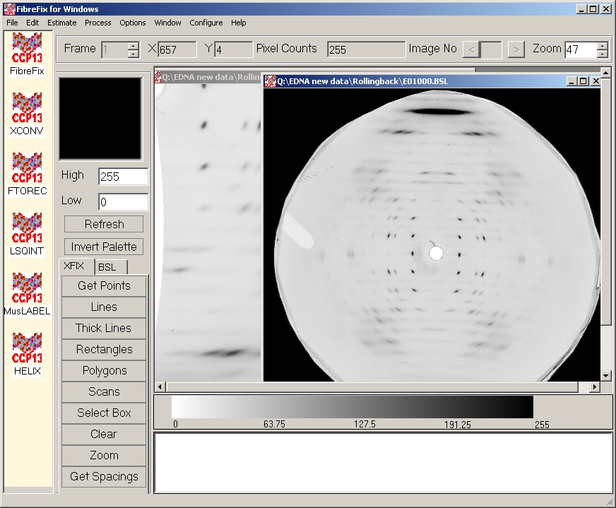
The FibreFix Main Window
The main windows consists of a menu bar, a tool bar, an image manipulation bar, an image display windows, a program startup panel and a message windows for displaying output from the processing program.
The integrated function is realized by the program startup panel, which can dynamically group CCP13 programs together. In the version 1.2, six applications have been developed and included in FibreFix. They are: FibreFix, XCONV, FTOREC, LSQINT,HELIX and MusLABEL.
The tool bar is used to display the current frame number and enables to change the frame for multiple image file. It also includes the (x,y) coordinates of the mouse position and the value at the point as well as Image No field which indicates the current image number. As soon as a file has been loaded and specified, the image number box Image No become active and enables to switch among the images.When the first image is displayed on the whole frame, the image number box is numbered zero. Zoom box enables to Zoom in or Zoom out the image.
On the image manipulation tool bar, there are the image magnification area, two text boxes for specifying the current display thresholds of the value of the image, an Invert Palatte push button for inverting the current palette, a Refresh push button for refreshing the display and a set of image manipulation functional buttons such as Point, Lines, Thick Lines.
The File Menu
1. Opening New Window
Multiple image area can be opened by selecting the New item under the File menu Option. This enables to open multiple images.
2. Opening a BSL Image
An image can be opened either by selecting the Open Image item under the File menu or by drag the image file from File Explorer. Fibre Fix open all the image formats supported by XCONV.
- Click the Open File menu to open the Open File dialog.
- Use the Open File dialog to browsethe image you want to open.
- Click the [OK] button to close the dialog and the image will be displayed on screen.
The following file types are allowed:
- float - float
- int - unsigned int
- short - unsigned short
- char - unsigned char
- smar - small MAR image plate (1200 x 1200)
- bmar - big MAR image plate (2000 x 2000)
- fuji - Fuji image plate (2048 x 4096)
- fuji2500 - BAS2500 Fuji image plate (2000 x 2500)
- rax2 - R-Axis II image plate
- rax4 - R-Axis IV image plate
- psci - Photonics Science CCD
- riso - RISO file format
- tiff - TIFF (8,12,16-bit greyscale with all Compression type)
- ESRF Id2(KLORA) - ESRF Data Format
- LOQ 1D - one dimensional ASCII data files recorded at LOQ
- LOQ 2D - two dimensional ASCII data files recorded at LOQ
- SMV - used by ADSC CCD detectors (8 bit unsigned, 16 bit unsigned, 32 bit signed integer, 32 bit float)
- ESRF Id3 -ESRF Data Format
- BRUKER -Area detector Frame format Siemens/Bruker file format (8 ,16 or 32 bits per pixel)
- Mar345-MAR345 Image Plate (File extension mar1200, mar1800, mar1600,mar2400, mar2000, mar3000, mar2300, mar3450)
- BSL - The BSL file format is described in the BSL manual.
- ILL_SANS -ILL-SANS Treated data formats.
Multiple file
Multiple file can be selected in the FibreFix. To select multiple files, the user must hold down the CTRL key while clicking the files to select. Consecutive files can be selected by clicking the first file to select and then, while holding down the SHIFT key, clicking the last file to select. You can use the multiselection feature to select multiple files in the FibreFix and perform operations on all the files selected as multframe BSL file. All the selected files should be same format and same dimension.
3. Saving Images
An image can be saved by selecting the Save Image File menu and saved as BSL file (header file + data file) , TIFF file , BMP or JPG image file.
- Click the Save Image File menu to open Save File dialog .
- Use theSave Options dialog to select directory and file type.
- Enter the filename of your choice.
- Select a file type with either the ".jpg"or ".bmp" file type.
- Click the [Save] button. This will check for an existing file withthe same namebefore saving a file and prompt you whether you wish to overwrite the file.
- Then the image will be saved to disk.
4. Opening Next Frame.
The next fame from a multi-frame file opened either byselecting Next Frame under file menu or by scrolling the frame number on the top window.
5. Opening Frame
User can loads a specified frame from a multi-frame file. by selecting Goto Frame under file menu or by scrolling the frame number on the top window.
6. Close Image
An image can be closedby selecting the Close item under the File menu.
7. Exit
On the File menu, click Exit, exits the program.
The Edit Menu
1. Setting parameter
Image parameters can be set by selecting the Parameter item under the Edit menu Option.
- Click the Parameter Edit menu to open the Parameter dialog.
- This interface is used to specify wavelength, sample to detector distance, detectorcentre and orientation, twist tilt, sample tilt and Calibrant d-spacing.
- The wavelength need specify in angstroms, sample to detector distance and detectorcentre are in pixels and orientation, twist, tilt, sample tilt in degree.
- Click OK or APPLY to set the values.
2. Object Editor dialog
The Object Editor dialog popup when selecting Object item under the Edit menu Option. This interface handles some of the items, which can be collected from the data: points, rectangles and polygons. These items can be selected by using mouse one at a time or with Shift and mouse or Ctrl and Mouse. The selected object can be delete form the list of objects.
3. Line Editor dialog
The Line Editor dialog popup when selecting Line item under the Edit menu Option. This interface handles some of the items which can be collected from the data: points, rectangles and polygons. These items can be selected by mouse one at a time or with Shift and mouse or Ctrl and Mouse. The selected Line can be delete form the list of Line object.
4. Scan Editor dialog
The Scan Editor dialogpopup when selecting Scan item under the Edit menu Option.
This interface handles some of the items which can be collected from the data: points, rectangles and polygons. These items can be selected by mouse one at a time or with Shift and mouse or Ctrl and Mouse. The selected Scan can be delete form the list of Scan object.
5. Celldialog
The Cell Editor popup whenselecting Cell item under the Edit menu Option. This interface is used to specify unit cell lengths and angles and the missetting angles of the unit cell away from the fibre axis.
The cell parameters can be used to generate reciprocal lattice points which are listed and mapped onto the diffraction pattern within the specified resolution range.
The Estimate Menu
1. Centre estimation
The centre of the pattern is estimated using the objects(points) created by points, rectangles, and polygons. The programme need minimum three point to estimate the centre. If more than three points available, the estimation is made by fitting a circle to the points.
If the wavelength or calibrant spacing have been specified using the Parameter Editor, the option is given to calculate the sample to detector distance.
2.Rotation estimation
The rotation of the pattern is estimated using a pairs of objects(points) created by points, rectangles, and polygons.
It is usually sufficient to select one or two pair of objects related by mirror symmetry across the meridian as the rotation can be refined later.
3. Tilt estimation
The tilt of the sample is estimated using a pairs of objects(points) created by points, rectangles, and polygons.
It is usually sufficient to select one or two pair of points related by mirror symmetry (for an untilted sample) across the equator as the tilt can be refined later.
The Process Menu
1. List Objects
This reportsthe wavelength ,Specimen-to-detector distanceDetector centre coordinates ,Detector rotation, twist and tilt, Specimen tilt angle when selecting List Object item under the Process menu Option.
2. Plot Lines
This popups a XFIX plotwindow and plot the lines when selecting Plot Lines item under the Process menu Option.
3. Plot Scans
This opens a XFIX plotwindow and plot the scans when selecting Plot Scans item under the Process menu Option.
XfixPlot window
This window isused to display the line and scan plots.
This window has option menu bar, The File menu has option to save the line data as 1-Dimension BSL or txt file, or image as JPG or BMP. The edit dialoghas option to set axis parameter X-axis starting and last channels and Y-axis Thresholds. Also there is a scroll number to select the lines and scans. For scan there is another option the select scanning method as“Azimuthal Scan “ or “Radial Scan”. Azimuthal Scan causes subsequently plotted scans to be integrated radially and the integrated values to be plotted as a function of angle. Radial Scan causes subsequently plotted scans to be integrated azimuthally and the integrated values to be plotted as a function of radius.
Channel and Plot Thresholds Selection
When a line/scan is plotted the distance between the start and end points of the line is divided into a sequence of channels, the length of a channel corresponding to the size of a data pixel. The values placed into the channels are found by interpolation of the data values. When the data for the line are plotted, the thresholds for the plot will be the minimum and maximum channel values present in the selected channels. If necessary, these can be altered by entering the appropriate values into the Min and Max textbox.
4. Refine
This popup the Refine Dialog by selecting Refine item under the Process menu Option.
The parameters for the refinement can be chosen and clicking on "OK" starts the refinement.
The refinement algorithm uses the current image as data, mapping the coordinates of the image into the four quadrants of reciprocal space in order to compare the data in the quadrants and minimize the variance between quadrants.
This means that the current image should be carefully chosen (not too big, but not so small that there is little contrast in the image, not too close to the equator if sample tilt is being refined but the intensity on the image should be present on all four quadrants of the image).
5. Background
There are three methods for estimating the background component of the diffraction pattern using XFIX:
(a) Paul Langan's "roving window" method.
(b) Calculation of a circularly-symmetric background.
(c) Calculation of a "smoothed" background through iterative low-pass filtering based on the method of M.I. Ivanova and L. Makowski (Acta Cryst. (1998) A54, 626-631).
(b) Calculation of a circularly-symmetric background.
(c) Calculation of a "smoothed" background through iterative low-pass filtering based on the method of M.I. Ivanova and L. Makowski (Acta Cryst. (1998) A54, 626-631).
These can be selected from the process menu by clicking on "background". All three methods require the user to input the pattern centre and the extent of the pattern (minimum and maximum radii in pixel units) in relation to the centre. Pixel values outside these limits will be ignored in the background estimation. If the diffraction pattern is not circular and centred around a single point, then it is possible to discard values less than a user-input minimum so that, for example, all values less than or equal to 0.0 are ignored in the background calculation. By using the BSL program from the NCD sofware suite , it is possible to mask the areas of the image that are not of interest (for example setting unwanted pixel values to a large negative value) and discarding these values in the background calculation.
The details of the different background estimation techniques are discussed below. In each case, once processing is completed, the user is prompted to view the calulated background. This will open a new XFIX interface with a 2-frame BSL file loaded (of filename specified by the user). The first frame in this file is the estimated background and the next frame is the diffraction data with the calculated background subtracted. This provides a visual indication of the "goodness of fit" of the calculated background. The calculated background in frame 1 of the file can then processed further using any of the three background estimation techniques. In this way, different background subtraction methods can be used successively if desired. Finally, the data-background frame can be used with a data fitting program such as LSQINT to measure the reflection intensities.
5.1 Roving window method
The roving window background subtraction method of Paul Langan estimates the background by moving a window (of size input by the user) across the collected data. The pixel values within this window are sorted and those in the user-selected range are taken as background (except pixel values lying outside the pattern extents or specified by the user as values to discard). The average pixel value within this range is then assigned to be the estimated background at the centre of the window. Fiinally, a smoothing spline under tension is fitted to fill in the gaps between window centres. The following parameters must be input by the user in the Roving window dialog.
- The pattern centre in X and Y (values in pixel units).
- The pattern extents taken radially from the centre (values in pixel units).
- Pixel values to discard.
- The window width and height (values in pixel units). The window will be of size 2*width+1 in X and 2*height+1 in Y.
- The separation of the window centres in X and Y (values in pixel units).
- The start and end positions in the sorted pixel list for selecting pixels corresponding to the background (expressed as a percentage of the total number of pixels in the window).
- The smoothing and tension factors for the spline fitting.
- The output BSL file name.
5.2 Circularly-symmetric background
A circularly-symmetric background can be formed by the radial binning of pixel values followed by averaging those pixel values lying within a specified range. This average value is assigned to the particular radius and a smoothing spline under tension is fitted to yield the estimated background. The following parameters must be input by the user in theCircularly-symmetric dialog
- The pattern centre in X and Y (values in pixel units).
- The pattern extents taken radially from the centre (values in pixel units).
- Pixel values to discard.
- The increment for radial binning (in pixel units).
- The start and end positions in the sorted pixel list for selecting pixels corresponding to the background (expressed as a percentage of the total number of pixels corresponding to the radial bin).
- The smoothing and tension factors for the spline fitting.
- The output BSL file name
5.3 Smoothed background - Iterative low-pass filtering
This method of background subtraction is based on that of M.I. Ivanova and L. Makowski (Acta Cryst. (1998) A54, 626-631). It takes advantage of the fact that the background of a fibre diffraction pattern is typically composed of lower spatial frequencies than the diffraction maxima. Hence an iterative low-pass filter can be applied to separate the two components on the basis of their frequencies. The estimated background depends on the frequency limit of the filter in both X and Y.
The application of the low pass filter is achieved by the convolution of the observed diffraction pattern with a box car or gaussian function (the smoothing function) having an average value of unity taken over the number of pixels it occupies and a value of zero elsewhere. This function is convoluted with the real data at each pixel within the pattern limits (excluding pixels that are specified by the user as to be discarded). The result of applying this filter is an overestimated background, containing some intensity from the diffracted maxima. This overestimated background is then subtracted from the real data to leave the diffraction maxima whose intensities are now underestimated. Positive pixel values in the image resulting from this subtraction are then subtracted from the original data to yield the next estimate of the background. This is then convoluted with the smoothing function and the procedure is repeated, with images of the original data minus estimated background providing a visual indication of the "goodness of fit" of the estimated background. The procedure is illustrated graphically in one-dimension in Figure 1 below.
There are problems that exist with this method of background estimation at the edge of the pattern where information cannot be obtained for the convolution. This can lead to edge effects (typically an underestimation of the background) which become more pronounced with each cycle of filtering. In this case, it is possible to import a background calculated by another method to be used as the final background estimate at the edges of the pattern. This is then left as constant throughout each cycle of filtering. The backgrounds calculated by the different methods are then merged by fitting a smoothing spline under tension.The following parameters must be input by the user smooth dialog.
- The pattern centre in X and Y (values in pixel units).
- The pattern extents taken radially from the centre (values in pixel units).
- Pixel values to discard.
- Whether to use a box car or gaussian as the smoothing function.
- The box car size or gaussian full-width-half-maximum (FWHM) (values in pixel units).
- The number of filtering cycles.
- Whether to apply the smoothing function / filter at the edge of the pattern.
- The background to be imported if the filter is not to be applied at the edge of the pattern.
- Whether to merge the backgrounds calculated by different methods.
- The smoothing and tension factors for spline fitting and the weight to be applied to the imported background in relation to the "smoothed" background.
- The output BSL file name.
Once the background estimation process has been completed, the user will be prompted to view the estimated background and original pattern minus estimated background as described above. This will open a new XFIX interface ( this may take a few seconds). Once the estimated background has been inspected, the user may then choose to perform more iterations of filtering. Hence it is possible to view the estimated background after each iteration if desired.
Figure 1: An illustration of the results of applying an iterative low-pass filter to the observed diffraction data.
(a) shows the current estimate of the background. On the first iteration, this is the recorded data.
(b) shows the result of "smoothing" the current background in (a) by applying a low-pass filter (ie. by convoluting the data in (a) with the smoothing function).
(c) shows the result of subtracting (b) from the original data.
(d) shows the result of subtracting positive values in (c) from the original data. (d) is now set to the current background and the procedure is repeated.
5.4 Rolling ball background
A rolling-ball background method removes a smooth continuous background from a two-dimensional image. Based on the imaging program being developed by Wayne Rasband at National Institutes of Health, USA (http://rsb.info.nih.gov/ij/). Rolling ball algorithm inspired by Stanley Sternberg's article, "Biomedical Image Processing", IEEE Computer, January 1983. It rolls the ball (actually a square patch on the top of a sphere) on a low-resolution (by a factor of 'shrinkfactor' times) copy of the original image in order to increase speed with little loss in accuracy. It uses linear interpolation to find the points in the full-scale background given the points from the shrunken image background. Also it uses linear extrapolation to find pixel values on the top, left, right, and bottom edges of the background.
6. Ftorec (Image space to reciprocal space transformation)
This popup the Ftorec Dialog by selecting Ftorec item under the Process menu Option. FTOREC is designed to take all or part of a diffraction image and transform this portion of the image into reciprocal space.
Click here to find out more about Ftorec
7. Lsqint (Fibre diffraction integration program)
The LSQINT function provide an automatic method for the integration of intensities for fibre diffraction data. This will handle patterns which are largely crystalline in nature, or patterns which have continuous layerlines, sampling only occurring parallel to the Z axis. More than one lattice can be fitted in a single pattern.
Click here to find out more about Lsqint
The Options Menu
Palette
This contains options for a grey scale and various colour representations of the pixel values.
Magnification
This contains options for the factor applied in the magnification window.
Line Colour
This popup Colour dialog Box the selected colour is use to draw the point, rectangles, line scan and circles.
Lattice Point Colour
This popup Colour dialog Box the selected colour is use to draw lattice points.
Log Scale
This causes subsequent threshold changes to scale the data on a logarithmic scale.
Interpolate
This causes subsequent images to be interpolated to fit the current image window size. This happens automatically for select images.
Show Lattice Points
This causes subsequently generated lattice points to be drawn onto the current image. If there are any lattice points in memory, these will be drawn immediately.
Generate Lattice points/ Generate Lattice rings
This causes subsequently generated lattice points or ring to be drawn onto the current image.
Show cursor cross
This causes cross line across the mouse point on the image.
Show log file
This enables to hide or view the processing information at the bottom of the XFIX.
Window Menu
Show all the multiple image document on the Windows desktop as Horizontally or Tile Vertically or Cascaded windows.
The Help Menu
The HTML help documents are displayed in your current Internet Web browser.
Manipulation bar
Image Thresholds Selection
The threshold values for displaying the current image can be set by editing the threshold text fields (labelled "High" and "Low") and hitting <return>. When an image is first loaded, the thresholds are set to the maximum and minimum values in the data for that image. By Clicking the Right-hand mouse and then by dragging up ,down ,left right threshold can be change interactively.
Inverting the Current Palette
The "Invert Palette" button reverses the colour scale of the current palette.
Refreshing the Image Display
The "Refresh" button can be used to redraw the image windows. This can be useful if another application has modified the colour map or if it is desired to erase circles or crosses drawn by FIX.
Data Collection Tools
To facilitate collection of various data items from the current image, a set of buttons is provided which determine the behaviour of the mouse buttons and pointer.
Points : Clicking the left-hand mouse button one can create points.
Lines : Clicking at starting point and ending point one can create lines.
Thick Lines: This is similar to "Lines" mode except that the line is now considered to have a width and is drawn as a rectangular box. Clicking at starting point and the ending point create a line then by creating another line vertical to the first line one can create a thick line.
Rectangles : Clicking at stating point and ending point one can create Rectangles. Then centre of gravity of the Rectangle will add to the image object and display object number. Centre of gravity is achieved by averaging data values along the perimeter of the rectangle to obtain a background value. This value is then subtracted from data point’s interior to the rectangle and the centre of gravity of the modified values is calculated.
Polygons : This is similar to "Rectangle" mode except that the left-hand mouse button crates a vertex; the right-hand mouse button closes the polygon. The centre of gravity for Polygons will add to the image object and display object number. Centre of gravity is achieved by averaging data values along the perimeter of the rectangle to obtain a background value. This value is then subtracted from data point’s interior to the rectangle and the centre of gravity of the modified values is calculated.
Scans:Clicking at stating point angle and radius and the ending angle and radius one can create Scan. Radii are measured from the pattern centre as defined in the Parameter Editor and angles are positive going anticlockwise on the image.
Select Box
This is essentially similar to "Rectangle" mode except that the rectangle chosen is become as current image. This image can be zoom-in and zoom-out and set Thresholds independent to the main image. Selected image is used in refinement process.
Zoom
When selected the zoom button one can zoom-in and zoom-out by clicking right mouse dragging the mouse pointer. The current zoom factor is displayed on the Zoom Text on to top window.
Get spacings
When selected the Get spacings one can estimate values of the Bragg spacing (d) of a peak, as well as the real space of the radial (1/R) and axial (1/Z) positions of the peak. These values will appear in the text box at the bottom of the FibreFix window.
BSL manipulation Tools
| ADC | Add a constant to a selected range in spectrum. |
| ADD | Weighted addition of two images. |
| ADF | Add sets of frames together in a time series. |
| ADN | Add and normalise image using a calibration file. |
| ASP | Apply aspect ratio. |
| AVE | Average a series of images. |
| BAK | Background subtraction of an image and correct background image using a calibration file |
| CAL | Calibration file plotting by dividing by frame exposer length |
| CEN | Estimate Center from four points or Center the image by adding extra coloms and rows |
| CHG | Change a selected value in an image. |
| CIN | Circular integration. |
| CLR | Clear Screen Drawing |
| CUT | Cut part of an image into a smaller image. |
| DIC | Divide a selected region of an image by a constant. |
| DIN | Divide and normalise image using a calibration file. |
| DIV | Weighted division of two images. |
| EXP | Exponentiate data values. |
| HOR | Perform a horizontal integration in a selected region. |
| ITP | Interpolate a 2-D iamge. |
| LOG | Calculate natural or base10 log of image. |
| MIR | Mirror the four quadrants of an image.. |
| MUC | Multiply a selected region of an image by a constant. |
| MUL | Weighted multiplication of two images. |
| MUN | Multiply and normalise image using a calibration file. |
| PAK | Pack an image into smaller dimensions by averaging and or Merge several small frames into one large image file. |
| PLA | Play move on time series. |
| POW | Raises image to specified power. |
| RIN | Radial scan and integration. |
| ROT | Rotate an image. |
| SEC | Perform sector integration. |
| SER | Make time series of image.. |
| SUN | Subtract and normalise image using a calibration file. |
| SUM | Sum a series of images. |
| TIP | Time series intensity plot. |
| VER | Perform a vertical integration in a selected region. |
| ZER | Set all negative values in an image equal to 0.0. |
Procedure for parameter determination using XFIX. by T. Forsyth
See following steps below. At all stages you may make measurements on the main image, or any part of it that you have zoomed in on (note there is a limit to the number of zoom boxes). Remember to change between "zoom" and "points" modes when you want to make interactive measurements from the image.
(i) Enter the wavelength & sample-detector distance under Edit/Parameters. Note that the sample-detector distance should be in pixel units. If you wish to use a calibration ring to determine this distance, see below.
(ii) Get rough values for the centre by measuring points on a salt ring, for example. If there isn't a salt ring, take four symmetry related reflections/diffraction features. Then go to Estimate/Centre. You will be asked if you want to calculate the sample-detector distance - say no unless you are dealing with a calibration ring (if so, you need to have placed the d-spacing for this ring under Edit/Parameters).
(iii) Get rough value for the rotation of sample relative to detector. Collect points in pairs, each pair containing symmetry related points on either side of MERIDIAN. Go to Estimate/Rotation.
(iv) Get rough value for the tilt of the sample relative to the x-ray beam. Collect points in pairs, each pair containing symmetry related points on either side of EQUATOR. Go to Estimate/Tilt. Remember this is a sensitive calculation (tangent changing very fast) where small measurement errors have a substantial effect. Your initial value may not be that good.
(v) Now refine the parameters (see Process/Refine). The refinement works by minimising the variance of the current selected region for all four quadrants (as defined in reciprocal space), and then using a downhill simplex algorithm for refinement. It usually works well but you have to be careful.
In Select-Box mode select a small(ish) box that looks promising. I have always found that the best approach is to refine centre & rotation first using a zoom box with clear features on all four quadrant, in a region that is not specifically affected by tilt. Then go to Process/Refine and activate "centre" and "Detector rotation", followed by "OK". If the selected region is not too large, the refinement will be quite quick.
Following this choose a region of the pattern for which tilt is clearly important (usually close to meridian, fairly high in Z) and for which symmetry related data are available in all four quadrants. Go to Process/Refine and activate "Specimen Tilt" only, followed by "OK".
Once you have these, you can try to refine things together. The last step is to try detector tilt & twist.
(vi) Once you have the parameters well determinedyou can try the background subtraction - eg (Process/Background) and then proceed to the RZ mapping step in FTOREC.

Diamond Light Source is the UK's national synchrotron science facility, located at the Harwell Science and Innovation Campus in Oxfordshire.
Diamond Light Source Ltd
Diamond House
Harwell Science & Innovation Campus
Didcot
Oxfordshire
OX11 0DE
Copyright © Diamond Light Source. Diamond Light Source® and the Diamond logo are registered trademarks of Diamond Light Source Ltd
Registered in England and Wales at Diamond House, Harwell Science and Innovation Campus, Didcot, Oxfordshire, OX11 0DE, United Kingdom. Company number: 4375679. VAT number: 287 461 957. Economic Operators Registration and Identification (EORI) number: GB287461957003.