Instruments by Science Group
Science Group Leader
Robert Rambo
Email: [email protected]
Tel: +44 (0)1235 56 7675
MusLABEL: A Diffraction and Labelling Simulation Program for Striated Muscles.
by John M. Squire & Carlo Knupp.
Please Email [email protected] to report bugs and problems.
Contents
Introduction
X-ray fibre diffraction has already proved invaluable in elucidating the structure of muscle, and with ever improving synchrotron sources and the development of new and sophisticated time-resolved detectors, fibre diffraction is likely to continue to have a major role in further advancing our understanding of muscular function.
However, the interpretation of X-ray diffraction patterns is not easy. To understand a muscle diffraction pattern, it is often useful to explore different structural models, calculate their diffraction patterns and see how these patterns change when some components of the model are moved. Diffraction patterns can be very sensitive to small changes in the model structure, and the final aim of this exploration is to recreate a structure that produces a diffraction pattern which is the same as that recorded experimentally.
MusLABEL has two different kinds of function. In one application it can simulate the kinds of diffraction pattern given by different helical structures such as myosin filaments, actin filaments and the troponin array on actin filaments. As part of this first role, like the program HELIX which is a subset of the MusLABEL program, it can also simulate the diffraction patterns from molecular structures like DNA, or the a-helix, or the collagen 10/3 helix (see the document file for HELIX to find out how to explore these molecular structures).
A great deal is known about the structures of myosin and actin filaments and about the different A-band lattice types that occur in different striated muscles, but questions are still open as to how myosin heads and other myosin associated proteins (e.g. C-protein) interact with actin filaments. One way of thinking about these interactions is to consider the myosin heads and the other myosin proteins as labelling the actin monomers with which they interact. In fact, much of their mass is shifted towards specific positions around the actin filaments, and a diffraction pattern can be calculated from them.
The second kind of application of MusLABEL is to calculate the labelling positions of myosin heads or myosin associated proteins such as C-protein interacting with actin, and then to compute and display the diffraction pattern obtained just due to that labelling pattern. It does not simulate the diffraction pattern from the whole muscle A-band – something which can be done using other programs such as MOVIE.
Before calculating the labelling positions, it is necessary to define the sarcomere structure by specifying the symmetry and the dimensions of the myosin and actin filaments. This can be achieved by inputting a series of parameters through the MusLABEL graphical user interface. In addition, it is also possible to input as parameters the axial and azimuthal extents to which the myosin heads or myosin associated proteins can move to reach the actin filament, as well as the position and the extent of a target location around the actin filament assuming that the azimuthal orientation of an actin monomer is important in determining how easily a myosin head or C-protein can attach to it. The program will then do three things: it will show which actin monomers have become labelled, it will indicate what percentage of the available heads or C-proteins have found binding sites on actin and it will calculate the diffraction due to the labelling pattern. The program makes no attempt to simulate the effects of head shape which can be done in other programs such as MOVIE.
This manual is intended to give a general illustration of how to use MusLABEL. It describes the type of parameters required by the program along with a worked example.
This program was created between 1987 and 2004 by John Squire and Carlo Knupp at Imperial College London and Cardiff University, and is available for download, along with HELIX, from this website. It has already been used in an earlier form in a number of publications:
Squire, J.M. and Harford, J.J. (1988) "Actin filament organisation and myosin head labelling patterns in vertebrate skeletal muscles in the rigor and weak?binding states" J. Mus. Res. Cell Motil. 9, (1988), 344-358.
Squire, J.M. (1992) "Muscle filament lattices and stretch-activation: The match/ mismatch model reassessed" J. Musc. Res. Cell Motil. 13, 183-189.
Squire, J.M., Luther, P.K. & Knupp, C. (2003) "Structural evidence for the interaction of C-protein (MyBP-C) with actin and sequence identification of a possible actin-binding domain." J. Mol. Biol. 331, 713-724.
Installation
MusLABEL has been developed for Microsoft Windows 98, and XP using Visual Basic 6.0. For the program to run, it is necessary to have the Visual Basic 6.0 run-time environment installed. This environment can be freely downloaded from the Microsoft website and can be installed, if it is not already present, by following the instructions provided by Microsoft.
In addition a library file named comdlg32.ocx may be needed. This file can be downloaded from a number of web sites (e.g. ftp://ftp.desy.de/pub/herab/rich/databases/comdlg32.ocx). Note if this doesn’t work, it maybe that your operating system needs another version of this file (same name though). Please search the net with Google, and then try a number of them.
This library file should be copied to the same directory that contains MusLABEL.exe.
After copying this file it is possible to start the program by double-clicking on MusLABEL.exe.
To access this help file from within the program, the file named MusLABEL.hlp must be stored in the same directory as MusLABEL.exe.
If the installation of MusLABEL fails, advice may be sought by emailing [email protected].
Parameters of a helix
The symmetry of a helical structure can be defined in terms of a number of parameters as illustrated in Figure 1(a). These include the subunit axial translation (h), the pitch of the helix (P), the repeat of the helix (C) if the number of subunits in a pitch is not an integer, and the radius of the helix (r). The number of subunits in one pitch is clearly N = P/h, and since the helix turns through 360° around the helix axis in a complete pitch, the amount turned from one subunit to the next is j = 360°/ N, an angle which we term the azimuthal rotation angle between subunits. As an example, the structure of the B form of DNA has exactly 10 sugar-phosphate-base subunits along one strand in a complete pitch length. This might be written as a 10/1 or 101 helix. The subunit axial translation is 3.4 Å, the pitch is 10 x 3.4 Å, and the azimuthal rotation angle between subunits is 360/10 = 36°. Because there is a whole number of subunits in one pitch, in this case the repeat C is the same as the pitch P.
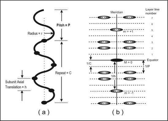
Figure 1: (a) Parameters of a helical structure (in this case a 5/2 or 52 helix, i.e. S=5 and T=2) and (b) the sort of distribution of diffracted intensities that is obtained from the helix in (a). The 1st meridional peak (m = 1) is on the 5th layer-line (i.e. S=5) and the strongest peaks close to the meridian are on the 2nd layer-line (i.e. T=2) and related positions (layer-lines at m ± 2).
The form of the helical diffraction pattern is a series of layers of intensity, so-called layer-lines, perpendicular to the helix axis (Figure 1(b)). The line in the diffraction pattern (by convention taken to be vertical) that is parallel to the helix axis and passes through the middle of the pattern (i.e. through the undiffracted beam direction) is termed the meridian and diffraction peaks on it are called meridional reflections. The horizontal line through the pattern centre is called the equator and this has equatorial reflections. The equator is part of the series of horizontal layer-lines. It is not appropriate here to give details of fibre diffraction theory, which are dealt with very well in other places (Holmes and Blow, 1965; Harford and Squire, 1996; Squire, 2000). Suffice it to say that, bearing in mind the reciprocal relationship between normal (real) space and diffraction (reciprocal) space, the positions of the layer-lines are related to successive orders of the repeat C of the helix. This means that, starting from the equator, they are at spacing related to 0/C (the equator), 1/C (the 1st layer-line), 2/C (the 2ndlayer-line) and so on. All of these layer-lines have intensity each side of the meridian, but not on the meridian, except for the layer-lines which correspond in spacing to orders of the subunit axial translation (h). These meridional intensities occur at axial positions related to m/h, where m is an integer, positive, negative or zero.
As a good rule of thumb, if one is dealing with a helix with S subunits in T turns of the helix, then the diffraction pattern can be drawn by counting out to the Sth layer-line at S/C from the equator and placing a meridional reflection there, and then counting out to the Tth layer-line at T/C from the equator and putting reflections each side of the meridian there. One can also count T layer-lines up and down from the meridional reflection on the Sth layer-line and put other off-meridional peaks there at the same radial positions as on the layer-line at T/C from the equator.
Finally, another important parameter of a helix is its radius (r). Because features in the diffraction pattern are at distances which are reciprocal to distances in the object, helices with a small radius will give off-meridional peaks at large reciprocal radii (R) along the layer-lines (they will be a long way from the meridian) and helices with a large radius will give peaks close to the meridian. Putting this the other way round, the radial position (R) of the peaks in the diffraction pattern can be used to determine the radius (r) of the helix.
Parameters for the MusLABEL program
Figure 2 shows the appearance of MusLABEL’s Graphical User Interface. It consists of several “Input boxes” in which the parameters necessary to build the myosin and actin filament models are to be typed, two “Picture boxes” in which the filament radial projections and the calculated diffraction pattern are shown, and two “Command buttons” to initiate the calculation either of the myosin filament structure coordinates or of the Fourier transform of the labelled structure itself. The first column of input boxes defines the parameters necessary to calculate the myosin head’s coordinates. However, there isn’t anything specific to myosin in the way these parameters are defined, and the monomer subunits of any generic filament can be created instead.
To calculate the myosin and actin filament coordinates and to define their labelling patterns, the following information should be provided:
The number of subunit levels: This number defines how many heads there are along any particular strand of the myosin (or of a generic) model.
The number of strands: This number defines the number n of strands in the myosin or generic model. The azimuthal separation of the strands on the surface of the filament is 360°/n. For example two strands will be separated azimuthally by 180° (=360°/2), three strands by 120° (=360°/3) and so on.
The axial separation of the subunits: This number defines the axial separation distance of adjacent monomers belonging to any one strand along the main axis, in Angstroms.
Rotation angle between subunits: This number defines the rotation angle, in degrees, between two adjacent monomers belonging to any one strand. This number defines the type of helical symmetry of the filament. For example if the filament is three-stranded with each strand possessing a 9/1 helical symmetry (i.e. with 9 heads in one turn) the rotation angle between adjacent monomers will be 1 * 360° / 9 = 40°. More generally an S/T helical symmetry (i.e. with S monomers in T turns) will require a rotational angle between adjacent monomers of T * 360° / S.

Figure 2: Appearance of the MusLABEL window (GUI). NB: the latest version of MusLABEL dated 27-7-04 has had an extra parameter added - bottom left - the subunit axial translation of the actin monomers in the actin filament. Otherwise the window is the same.
The radial position of the monomer centre or the myosin head radial position from the centre of the fibre: This number defines the distance, in Å, of the myosin heads from the centre of the backbone. In the case of a general filament model, it defines the distance of each monomer from the centre of the filament.
The size of the subunit radius: This number defines the radius, in Å, of each myosin head or, in the case of a general filament, of a subunit monomer. All heads or subunits are approximated to spheres of constant radius.
The azimuthal shift of the second strand: This parameter can be used only if the number of strands is set to 2. It defines the azimuthal shift, in degrees, of the second strand from its original position.
The axial shift of the second strand: This number can be typed only if the number of strands is set to 2. It defines the axial shift, in Angstrom, of the second strand from its original position.
The handedness of the strands: This information is necessary to define the handedness of the strands forming the myosin or the filament model. A right hand filament assumes the rotation angle between subunit to be positive. Conversely, a left hand filament assumes a rotation angle between subunit to be negative.
Actin helix pitch: This is the first of the parameters that define the six actin filaments surrounding the myosin filament and positioned at the vertices of a hexagon. Leaving this parameter to zero, is a signal to MusLABEL that only the diffraction pattern of the myosin filament (or the generic filament) must be calculated. If this parameter is used, it indicates the pitch of the actin filament helices surrounding a myosin. This pitch can vary between 700 and 770 Å. Its value should be about 735 Å for the actin filaments in vertebrate striated muscles (a slightly untwisted 13/6 helix) and about 770 Å for insect flight muscle (a 28/13 actin filament).
Figure 3: Lattice geometry looking down the fibre axis
Relative orientation of actin helices: This parameter, indicated in Figure 3 as r, defines the rotation angle in degrees between one actin filament and the next filament. The six filaments surrounding a myosin are enumerated anticlockwise from 1 to 6. With respect to an absolute frame of reference, the second actin is rotated by (60 + r)° degrees with respect to the first, the third actin is rotated by 2*(60 + r)° with respect to the first, the fourth actin by 3*(60 + r)° and so on. An angle r set equal to -60° generates six actin filaments with the same absolute orientation in the A-band lattice.
Number of residues per actin filament: This parameter defines the number of actin monomers in each filament.
Radius of actin filament surface: This parameter defines the radius of the actin filaments in Angstroms.
Filament separation: This parameter defines the distance between the myosin filament and any of the six surrounding actin filaments in Angstroms.
Extreme axial range of bridge: This parameter defines the extent to which the myosin head is allowed to move axially to search for the optimal actin monomer to label. In the side view of Figure 3, this parameter is indicated as Dz and the axial search is carried out between +Dz and -Dz. Dz is measured in Angstroms.
Extreme azimuthal range of bridge: This parameter defines the azimuthal extent to which the myosin head is allowed to move to search for the optimal actin monomer to label. In the top view of Figure 4, this parameter is indicated as Dq degrees and the axial search is carried out between +Dq and -Dq.
Extreme azimuthal extent of target: This parameter defines the azimuthal extent on the actin filament within which the myosin head is allowed to attach if it finds a suitable monomer. In the top view of Figure 4, this parameter is indicated as Df° and the actin target is between +Df and -Df.
Azimuthal offset of target area: This parameter defines the azimuthal offset on the actin filament which is the centre of the 2 x Df azimuthal range. In the top view of Figure 4, this parameter is indicated as f and is measured in degrees. In other words the target is at f ± Df relative to the myosin head origin.
Axial shift of myosin filament: This number specifies the axial shift between the myosin and the actin filaments in Å.
Myosin filament rotation: This number specifies the offset rotation angle, in degrees, for the myosin filament.
Figure 4: Defining the search range of a crossbridge
Actin filament rotation: This number specifies the offset rotation angle, in degrees, for the each actin filament.
Number of myosin heads to use: This parameter allows the selection of the number of labelling objects associated with each subunit of the myosin filament. This number can be 2 or 1. The number 2 will be chosen in the case of myosin heads (which come in pairs on each myosin origin), and 1 in the case of other myosin associated proteins such as C-protein.
Actin monomer radius: This parameter defines the radius of the monomers in the actin filaments in Å.
Select axially or azimuthally: For given values of Δ z, Δθ and ΔΦthe number of targets found to be available may well be greater than the number of myosin heads to be used. By selecting a minimum axial search, the targets chosen will be those at the smallest possible values of ΔZ that are within the 2 x Δθ azimuthal range. By selecting a minimum azimuthal search, the targets chosen will be those at the smallest possible values of Δθ that are within the 2 x Δz axial range. The check box shows a tick when the targets to be labelled are searched with minimum axial displacement.
Introducing the radial projection
Once the filament parameters have been defined, it is possible to calculate the coordinates of the myosin (or generic) filament alone by unselecting the draw actin lattice tick box and by pressing the Display Structure button. The filament is then represented in the right hand side “Picture box” as a radial projection.
A radial projection is a clever and convenient way of displaying in two dimensions the three-dimensional structure of a filament. Figure 2 shows how to create a radial projection of a 28/13 actin filament represented as two stranded helix in which each strand possesses 14/1 helical symmetry.
In Figure 5(a) an imaginary sheet of paper is wrapped around the filament, and the outwards-projected positions of the filament monomers are recorded on the paper (black marks). Successively, the sheet is unwrapped (Figure 5(b)), and the marks on the paper define the radial projection of the filament (Figure 5(c)). Monomers belonging to different strands are highlighted here by green and purple lines. This lines travel upwards from left to right describing a right hand helix. The lines leaving the radial projection on the right reappear immediately on the left to continue their course. This is because the left and right borders of a radial projection are actually the same border, as seen when the sheet is still wrapped around the filament (Figure 5(a)).
Figure 5: Illustration of the generation of a radial projection
Along a particular strand, for example the purple one, there are here exactly 14 monomers between the entry position on the left of the radial projection and the leaving position on the right. In other words there are 14 monomers in one turn of the strand and its symmetry is said to be 14/1. Note that, with this description of the 28/13 helix, the second strand also has 14/1 helical symmetry, but it is related to the first by an axial shift of 27.5 Å and a rotation around the helix axis of 192.86° (=360° – (13 x 360°/28)).
It is possible to change the filament image magnification and position within the box by changing the values of the “Input boxes” in the Filament Image Parameter frame.
By changing the value of the Scale Factor, we can set the magnification of the radial projection of the filament model.
Offset along X and Offset along Y change the origin position of the radial projection within the filament image picture box. These offset coordinates can be also changed by clicking on the arrows of the slide bars on the right and at the bottom of the filament image picture box (see figure 5).
Finally, the View Radial Projection from Outside the Filament check box, allow the selection of the observer’s point of view between the inside and the outside of the filament.
Calculating fibre diffraction patterns
Once the coordinates of the filament have been defined, the fibre diffraction pattern is calculated by computing a cylindrically averaged Fourier transform.
Figure 6: A 28/13 actin filament as a 1-start helix and positioning of the image
Before calculating the diffraction pattern, two important parameters should be set in the FT Image Parameter Frame. First it should be decided how many pixels are wanted in the Transform Image picture box. Here, a compromise should be made between the quality of the diffraction pattern (more pixels = better quality) and the time needed to calculate it (more pixels = longer calculation time). In addition, it has to be noted that if the transform image contains too few pixels, serious aliasing problems may arise that limit the quality of the transform image.
Secondly, it should be decided up to what resolution the diffraction pattern should be calculated. Since a diffraction pattern is described in reciprocal space, a smaller number for the maximum resolution means a diffraction pattern calculated to a higher radius. Once these parameters have been defined, the diffraction pattern is calculated by pressing the Calculate Fourier transform button (see an example of transform in figure 6).
The transform image greyscale ranges between 0 and 255, but these levels can be changed by altering the Max Intensity and Min Intensity Input boxes in the FT Image Greyscale Parameters Frame. After changing the greyscale thresholds, the transform image must be updated by pressing the Refresh Image Command Button.
Figure 7: Simulation of the diffraction from a 1 start 28/13 actin filament
Building models of sarcomeres
(1) Vertebrate Striated Muscles
A model of a sarcomere A-band can be easily set up using the MusLABEL graphical user interface. Initially, we need to define the symmetry and the dimensions of the myosin thick filament. For example, we can use the myosin symmetry associated with vertebrate striated muscles and create a 3-stranded myosin filament with three pairs of heads forming a crown repeating axially every 143 Å. To a first approximation, each strand possesses 9/1 helical symmetry, corresponding to a rotation angle between subunits of 40°. To minimise calculation times, we have carried out the calculations using 30 crown levels (Figure 8). The resulting radial projection is displayed in Figure 8 along with its calculated diffraction pattern to 60 Å resolution. The head shape has not being included in the MusLABEL armoury so details of the intensities along the layer-lines will not be correct. What the program does is to show where the layer-lines will be and which ones are likely to be strong just from the filament symmetry.
Figure 8: Simulation of the diffraction pattern from a single 3-stranded 9/1 myosin filament
Once the myosin filament has been created, we need to generate the actin filaments for vertebrate muscle. For these, we can choose a pitch of 735 Å, a value for the relative orientations of -60° (all actins with the same absolute orientation), an outer filament radius of 50 Å, a myosin to actin centre to centre distance of 270 Å, and a radius for each actin monomer of 24 Å. The result (Figure 9) is displayed by pressing the Display Structure command button. For display purposes only, the myosin filament is projected radially on to a cylinder of radius 270 Å (myosin to actin distance). The six actins, represented in red, are projected onto the same cylinder to facilitate the visual inspection of the labelled targets. Note that there are 7 actin filaments represented, but the extreme left hand and right hand filaments are the projection of the same actin filament.
Note that here and for any labelling pattern calculations it is imagined that the myosin head array is being viewed by an imaginary tiny observer looking from the axis of the myosin filament outwards towards the myosin head array on the filament surface and then beyond that to the surrounding actin filament array. To see this properly the View Radial Projection from Outside box should not be checked.
The effect of this is that the right-handed myosin head array, viewed from the inside, looks left-handed as in Figures 8 and 9, but the long-period right-handed helices of the actin filament appear right-handed since they are being viewed from outside.
Figure 9: Establishing the myosin filament array and viewing the surrounding actin filament lattice.
Figure 9 shows that the labelling pattern computation also allows the percentage of attached heads to be displayed. This number is given at the top of the structure window – in this case it is 78.6%. It is shown later that in insect flight muscle this number can vary with filament overlap even though the search parameters remain the same.
Figure 10: The labelling pattern in Figure 9, together with its computed diffraction pattern. The strong reflection on the meridian is the well-known M3 reflection at 143 Å. The strong extended layer-lines just above and below the equator are the ‘first’ actin layer-lines at about 367.5Å.
The parameters for insect flight muscle, here represented by the flight muscles in Lethocerus, are rather different from those in vertebrate striated muscles. Firstly the myosin filaments are 4-stranded, have a larger backbone radius, about 80 Å, and a different axial repeat (1160Å) after 8 crowns of heads compared with the vertebrate thick filaments (429 Å repeat after 3 crowns). As far as the actin filaments are concerned they have 28/13 helical symmetry, rather than the roughly 13/6 symmetry in vertebrate muscle. This means that the azimuthal rotation between actin subunits, if the diffraction pattern of the actin filament alone is being calculated (cf. Figure 7), is 360 x 13/ 28 = 167.14° (rather than 360 x 6/13 = 166.15° for vertebrate muscle). A further difference is the relative rotation between adjacent actin filaments. The A-band lattices in the two muscle types are compared in Figure 11(b and c). As seen in (b), the vertebrate actin filaments are thought to have the same absolute azimuthal orientation (they are in helical register), whereas in the insect flight muscle lattice there are systematic rotations of 60° (or 120°) between adjacent actin filaments. If actin filaments on diametrically opposite sides of the myosin filament have identical orientations then the rotation between adjacent actins around the myosin muscle be 120°, but there is evidence that there may
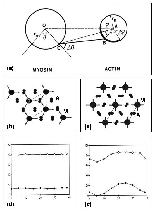
Figure 11. (a) Geometry of interaction of myosin heads from a site C on the myosin filament (left) to an actin site (B) on an adjacent actin filament (right) (after Squire and Harford, 1988; Squire, 1992; cf Figure 4). For a given head start position (C; defined by the angle q), the interaction geometry can be defined in terms of an azimuthal search limit (Dq) and a corresponding axial search limit (DZ; not illustrated) of the head, combined with the position of the actin site relative to the line CA joining the myosin head origin position to the actin filament axis. This is defined by the angles f and Df. The precise implications of the geometry in (a) depend very much on the lattice type that is involved. (b) The filament lattice arrangement (the simple lattice; see Luther et al., 1981) in bony fish muscle illustrating that the 3-fold symmetric myosin filaments (M) all have the same orientations as do all the actin filaments (A). (c) As for (b) but for the 4-fold symmetric myosin filament array in insect (Lethocerus) flight muscle. The myosin filaments (M) all have the same orientations at least locally in the Lethocerus A-band (although there may be different orientations elsewhere in the same myofibril giving a domain structure; Freundlich and Squire, 1983). However, the actin filaments (A) show systematic rotations. (d,e) The effects of applying the search parameters in (a) to the two lattices in (b) and (c) and then changing the axial positions of the actin and myosin filaments as would occur with changes in sarcomere length. Because of actin target area labelling (see Squire, 1972; Squire and Harford, 1988; Squire, 1992), the ease of attachment of a head to an actin site depends on the azimuth of the actin site. In (e), because the actin filament array matches the myosin head geometry (Wray, 1979), for a given set of head search parameters (results for two sets are shown in (d) and (e)), as the sarcomere length changes the probability of attachment also changes. Because the common periodicity in this case is 385 Å, the pattern in (e) repeats over this distance. Wray (1979) suggested that this lattice matching and mis-matching as the sarcomere length changes might be associated with the stretch-activation properties of asynchronous insect flight muscle. This possibility is supported by the response of vertebrate muscle in (d) where the level of attachment does not change significantly as the filament overlap changes. Figure from Squire et al. (2005).
be some 2-fold (i.e. 180°) randomness in the absolute filament orientations at any particular lattice point.
Figure 11 is from a paper currently in press (Squire et al., 2005) showing an example of the practical application of the MusLABEL program to particular muscle problems. In this case it shows how the two different A-band lattice geometries in vertebrate striated and insect flight muscles produce very different effects on the number of heads that can attach for a given set of head search parameters. An easy thing to do with MusLABEL is to set all the filament and search parameters and then to change the axial shift of the myosin filament in small steps (perhaps 10Å) and get the program to determine the number of attached heads. This is equivalent to exploring the effect of changes in sarcomere length on the labelling pattern. Figure 11(d) shows that the vertebrate lattice is such that the number attached changes rather little with changing sarcomere length, whereas in the insect flight muscle lattice (Figure 11(e)) the number changes periodically; a feature which may be related to the stretch-activation property of this muscle type (Wray, 1979).
The menu bar
Once a particular set of parameters hase been input into MusLABEL and all desired calculations have been done, the MENU bar of MusLABEL allows various options:
The MENU bar contains four entries: Open, Save, Exit, and Help.
Open allows the loading of a saved Parameter File, or of a Diffraction Pattern (Fourier transform) image. After opening a parameter file, MusLABEL calculates automatically the filament model coordinates and displays their radial projection.
Save allows the creation of a parameter text file containing the values from all input boxes, the creation of a bitmap (BMP) file containing either the filament image or the transform image and the creation of a text, comma-separated variable (CVS) file containing the target coordinates or the coordinates of the myosin/general filaments and of the actins. These coordinates are saved as cylindrical coordinates and consists of values for radius, angle (in degrees) and Z position for all monomers of the model. This file is saved in text format with CSV extension for easy loading with Microsoft Excel.
Exit terminates the program.
Help calls the help file.
Exercises
The features of the diffraction patterns are very sensitive to the parameters describing the model structures. Using MusLABEL, it is possible to explore the effects on the diffraction pattern when the structure parameters are changed. For example, starting from the parameter file describing a 28/13 actin filament (Figure 7), it is interesting to find out:
- What happens when the radius of the spheres representing the actin subunits is increased or decreased?
- What are the effects on the layer lines, when the number of subunits levels is changed?
- How do radial positions of the strong off-meridional reflections in the diffraction pattern change when the radial position of the centres of the monomers is varied?
- How does the pattern change when the axial separation of the monomers is changed?
- What is the effect of changing the pitch of the helix (e.g. by changing the rotation angle between subunits)?
Bibliography
Explanations of helical diffraction and other effects can be found in the articles:
“Fibre and Muscle Diffraction” by J.M Squire (2000) in “Structure and Dynamics of Biomolecules”, E. Fanchon, E. Geissler, L-L Hodeau, J-R Regnard & P. Timmins Eds., Oxford University Press,
"Time-resolved studies of muscle using synchrotron radiation". Harford, J.J.& Squire, J.M. (1997) Rep. Prog. Phys. 60, 1723-1787.
"Use of X-ray diffraction in the study of protein and nucleic acid structure" Holmes, K.C. & Blow, D.M. (1965) Interscience Publishing Company.
and in Chapter 2 of: “The Structural Basis of Muscular Contraction”, by Squire, J.M. (1981) Plenum press, New York and London .
Applications of MusLABEL (and its precursor programs) are described in
Squire, J.M. and Harford, J.J. (1988) "Actin filament organisation and myosin head labelling patterns in vertebrate skeletal muscles in the rigor and weak‑binding states" J. Mus. Res. Cell Motil. 9, (1988), 344-358.
Squire, J.M. (1992) "Muscle filament lattices and stretch-activation: The match/ mismatch model reassessed" J. Musc. Res. Cell Motil. 13, 183-189.
Squire, J.M., Luther, P.K. & Knupp, C. (2003) "Structural evidence for the interaction of C-protein (MyBP-C) with actin and sequence identification of a possible actin-binding domain." J. Mol. Biol. 331, 713-724.
Squire, J.M., Knupp, C., Roessle, M, AL-Khayat, H.A., Irving, T.C., Eakins, F., Mok, N.S., Harford, J.J. and Reedy, M.K. (2005) X-ray diffraction studies of striated muscles. In 'Puzzles of the sliding filament mechanism' (Ed. H. Sugi). Advances in experimental medicine and biology. Volume XXX, pp. yyy-zzz. Kluwer/ Plenum.
Other relevant papers are:
Squire, J.M. (1972) "General model of myosin filament structure II: myosin filaments and crossbridge interactions in vertebrate striated and insect flight muscles" J. Mol. Biol. 72,125-138.
Squire, J.M. (1997) “Architecture and function in the muscle sarcomere”. Curr. Opin. Struct. Biol. 7, 247-257.
Wray, J.S. (1979) “Filament geometry and the activation of insect flight muscle”. >Nature 280, 325-326.
Contacts
Carlo Knupp ([email protected])
Biophysics Group, Dept of Optometry and Vision Sciences, Redwood Building, Cardiff University, Cardiff CF10 3NB.
John M. Squire ([email protected])
Biological Structure & Function Section, Biomedical Sciences Division, Imperial College London, London SW7 2AZ, UK.

Diamond Light Source is the UK's national synchrotron science facility, located at the Harwell Science and Innovation Campus in Oxfordshire.
Diamond Light Source Ltd
Diamond House
Harwell Science & Innovation Campus
Didcot
Oxfordshire
OX11 0DE
Copyright © Diamond Light Source. Diamond Light Source® and the Diamond logo are registered trademarks of Diamond Light Source Ltd
Registered in England and Wales at Diamond House, Harwell Science and Innovation Campus, Didcot, Oxfordshire, OX11 0DE, United Kingdom. Company number: 4375679. VAT number: 287 461 957. Economic Operators Registration and Identification (EORI) number: GB287461957003.