Instruments by Science Group
Science Group Leader
Robert Rambo
Email: [email protected]
Tel: +44 (0)1235 56 7675
HELIX: A Helical Diffraction Simulation Program
by Carlo Knupp & John M. Squire
Please Email [email protected] to report bugs and problems.
Contents
Introduction
X-ray fibre diffraction is a very powerful method for determining the structure of polymers, both biological and synthetic. For example, X-ray fibre diffraction allowed the proposal of the famous Watson-Crick double helix model for the DNA molecule, which opened the way to modern genetics. It was also a fundamental tool used to solve or confirm the structures of all regular secondary folds of proteins (α-helix, β-sheet, collagen, etc).
Technological progress in recent years has resulted in the creation of powerful X-ray sources (e.g. synchrotrons) and of faster and better detectors that allow us to record viable X-ray diffraction patterns in periods of the order of milliseconds or less. This has made X-ray fibre diffraction an even more powerful tool with which to answer questions about molecular and atomic interactions within biological or synthetic polymers.
However, understanding the relationship between a polymer structure and the diffraction pattern generated from it is not a trivial task. This is especially true for newcomers to the field. HELIX is a didactic program designed for students and researchers who want to improve their understanding of the relationship between filament structure models and their diffraction patterns. It allows the construction of simple filament models through the input of a series of structural parameters via a user-friendly graphical user interface. It then calculates the filament diffraction pattern for visual inspection. It also allows the recording of the model filament coordinates along with their calculated patterns.
HELIX can be also extremely useful when a new diffraction pattern has been recorded experimentally from a novel polymer for which little information is available. In particular, HELIX allows rapid qualitative testing of different possible models for the unknown structure. The information obtained from such a preliminary analysis using HELIX can then be used to initiate more detailed model construction and refinement by other means.
This manual is intended to give a general illustration of how to use HELIX It describes the type of parameters required by the program along with a worked example.
This program was created between 2003 and 2004 by John Squire and Carlo Knupp at Imperial College London and Cardiff University, and it stems from MusLABEL, also available for download from this website.
Installation
HELIX has been developed for Microsoft Windows 98, 2000 and XP using Visual Basic 6.0. For the program to run, it is necessary to have the Visual Basic 6.0 run-time environment installed. This environment, distributed as vbrun60sp5.exe, can be freely downloaded from the Microsoft website and can be installed, if it is not already present, by following the instructions provided by Microsoft.
In addition a library file named comdlg32.ocx may be needed. This file can be downloaded from a number of web sites (e.g. ftp://ftp.desy.de/pub/herab/rich/databases/comdlg32.ocx).
This library file should be copied to the same directory that contains HELIX.exe.
After copying this file it is possible to start the program by double-clicking on HELIX.exe.
To access this help file from within the program, the file named HELIX.hlp must be stored in the same directory as HELIX.exe.
If the installation of HELIX fails, advice may be sought by emailing [email protected].
Parameters of a helix
The symmetry of a helical structure can be defined in terms of a number of parameters as illustrated in Figure 1(a). These include the subunit axial translation (h), the pitch of the helix (P), the repeat of the helix (C) if the number of subunits in a pitch is not an integer, and the radius of the helix (r). The number of subunits in one pitch is clearly N = P/h, and since the helix turns through 360° around the helix axis in a complete pitch, the amount turned from one subunit to the next is j = 360° / N, an angle which we term the azimuthal rotation angle between subunits. As an example, the structure of the B form of DNA has exactly 10 sugar-phosphate-base subunits along one strand in a complete pitch length. This might be written as a 10/1 or 101 helix. The subunit axial translation is 3.4 Å, the pitch is 10 x 3.4 Å, and the azimuthal rotation angle between subunits is 360/10 = 36° . Because there is a whole number of subunits in one pitch, in this case the repeat C is the same as the pitch P.
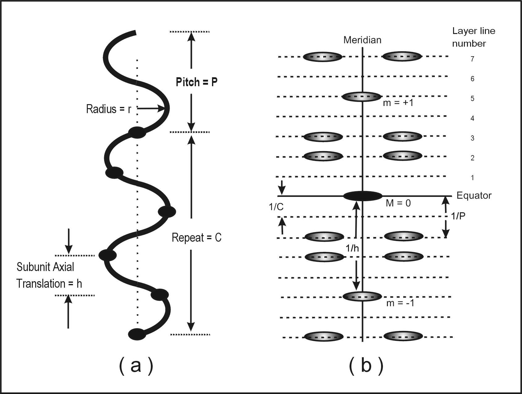
Figure 1: (a) Parameters of a helical structure (in this case a 5/2 or 52 helix, i.e. S=5 and T=2) and (b) the sort of distribution of diffracted intensities that is obtained from the helix in (a). The 1st meridional peak (m = 1) is on the 5th layer-line (i.e. S=5) and the strongest peaks close to the meridian are on the 2nd layer-line (i.e. T=2) and related positions (layer-lines at m ± 2).
The form of the helical diffraction pattern is a series of layers of intensity, so-called layer-lines, perpendicular to the helix axis (Figure 1(b)). The line in the diffraction pattern (by convention taken to be vertical) that is parallel to the helix axis and passes through the middle of the pattern (i.e. through the undiffracted beam direction) is termed the meridian and diffraction peaks on it are called meridional reflections. The horizontal line through the pattern centre is called the equator and this has equatorial reflections. The equator is part of the series of horizontal layer-lines. It is not appropriate here to give details of fibre diffraction theory, which are dealt with very well in other places (Holmes and Blow, 1965; Harford and Squire, 1996; Squire, 2000). Suffice it to say that, bearing in mind the reciprocal relationship between normal (real) space and diffraction (reciprocal) space, the positions of the layer-lines are related to successive orders of the repeat C of the helix. This means that, starting from the equator, they are at spacing related to 0/C (the equator), 1/C (the 1st layer-line), 2 /C (the 2nd layer-line) and so on. All of these layer-lines have intensity each side of the meridian, but not on the meridian, except for the layer-lines which correspond in spacing to orders of the subunit axial translation (h). These meridional intensities occur at axial positions related to m/h, where m is an integer, positive, negative or zero.
As a good rule of thumb, if one is dealing with a helix with S subunits in T turns of the helix, then the diffraction pattern can be drawn by counting out to the Sth layer-line at S/C from the equator and placing a meridional reflection there, and then counting out to the Tth layer-line at T/C from the equator and putting reflections each side of the meridian there. One can also count T layer-lines up and down from the meridional reflection on the Sth layer-line and put other off-meridional peaks there at the same radial positions as on the layer-line at T/C from the equator.
Finally, another important parameter of a helix is its radius (r). Because features in the diffraction pattern are at distances which are reciprocal to distances in the object, helices with a small radius will give off-meridional peaks at large reciprocal radii (R) along the layer-lines (they will be a long way from the meridian) and helices with a large radius will give peaks close to the meridian. Putting this the other way round, the radial position (R) of the peaks in the diffraction pattern can be used to determine the radius (r) of the helix.
Parameters for the Helix program
Figure 2 shows the appearance of HELIX’s Graphical User Interface. It consists of several “Input boxes” in which the parameters necessary to build a filament model are to be typed, two “Picture boxes” in which the filament radial projection and its calculated diffraction pattern are shown, and two “Command buttons” to initiate the calculation either of the filament structure coordinates or of the Fourier transform of the structure itself. To calculate the filament coordinates, the following information should be provided (refer to Figure 1(a) for definitions):
Figure 2: Appearance of the HELIX Graphical User Interface
The number of subunit levels: This number defines how many monomer subunits there are along any particular strand of the model. Generally this number should be a few times the number if subunits in a repeat, but should not be too large.
The axial separation of the subunits (h): This number defines the axial separation distance of adjacent monomers belonging to any one strand along the main axis, in Angstroms.
The number of strands (n): This number defines the number n of strands in the model. The azimuthal separation of the strands on the surface of the filament is 360/n degrees. For example two strands will be separated azimuthally by 180 (=360/2) degrees, three strands by 120 (=360/3) degrees and so on.
The azimuthal shift of the second strand: This parameter can be used only if the number of strands is set to 2. It defines the azimuthal shift of the second strand from its original position. An equivalent 2nd strand would be 180 degrees away from the first strand.
The axial shift of the second strand:This number can be typed only if the number of strands is set to 2. It defines the axial shift of monomers in the second strand relative to those in the 1st.
Rotation angle between subunits in degrees (j = 360° / N where N = P/h): This number defines the rotation angle between two adjacent monomers belonging to any one strand. This number defines the type of helical symmetry of the filament. For example if the filament is one stranded with a 14/1 helical symmetry (i.e. with 14 monomer subunits in one turn) the rotation angle between adjacent monomers will be 1 * 360 / 14 = 25.71 degrees. More generally an S/T helical symmetry (i.e. with S subunits in T turns) will require a rotational angle between adjacent monomers of T * 360 / S degrees.
The radial position of the monomer centre from the centre of the fibre (r): this number defines the radius of the filament model.
The size of the subunit radius in Angstroms: this number defines the radius (i.e. size) of a sphere representing each subunit. .
The handedness of the strands: This information is necessary to define the handedness of the strands forming the filament model. A right hand filament assumes the rotation angle between subunit to be positive. Conversely, a left hand filament assumes a rotation angle between subunit to be negative.
The radial projection
Once the filament parameters have been defined, it is possible to calculate the coordinates of the model filament by pressing the Display Structure button. The filament is then represented in the right hand side “Picture box” as a radial projection.
Figure 3: Explanation of a Radial Projection
A radial projection is a clever and convenient way of displaying in two dimensions the three-dimensional structure of a filament. Figure 3 shows how to create a radial projection of a two stranded filament in which each strand possesses 14/1 helical symmetry.
In Figure 3(a) an imaginary sheet of paper is wrapped around the filament, and the outwards-projected positions of the filament monomers are recorded on the paper (black marks). Successively, the sheet is unwrapped (Figure 3(b)), and the marks on the paper define the radial projection of the filament (Figure 3(c)). Monomers belonging to different strands are highlighted here by green and purple lines. This line travels upwards from left to right describing a right hand helix. The lines leaving the radial projection on the right reappear immediately on the left to continue their course. This is because the left and right borders of a radial projection are actually the same border, as seen when the sheet is still wrapped around the filament (Figure 3(a)).
Along a particular strand, for example the purple one, there are here exactly 14 monomers between the entry position on the left of the radial projection and the leaving position on the right. In other words there are 14 monomers (S) in one turn (T) of the strand and its symmetry is said to be 14/1.
Figure 4: Setting up a Model of a 2-start 14/1 helix simulating an actin filament
Notably, the parametric description of the filament model symmetry is not unique. Figures 4 and 5 show two different ways of creating the same radial projection of an actin filament. The demonstration of the equivalence of the two descriptions is left to the reader.
Figure 5: A 28/13 actin filament as a 1-start helix and positioning of the image
It is possible to change the filament image magnification and position within the box by changing the values of the “Input boxes” in the Filament Image Parameter frame.
By changing the value of the Scale Factor, we can set the magnification of the radial projection of the filament model.
Offset along X and Offset along Y change the origin position of the radial projection within the filament image picture box. These offset coordinates can be also changed by clicking on the arrows of the slide bars on the right and at the bottom of the filament image picture box.
Finally, the View Radial Projection from Outside the Filament check box, allow the selection of the observer’s point of view between the inside and the outside of the filament.
Calculating fibre diffraction patterns
Once the coordinates of the filament have been defined, the fibre diffraction pattern is calculated by computing a cylindrically averaged Fourier transform.
Before calculating the diffraction pattern, two important parameters should be set in the FT Image Parameter Frame. First it should be decided how many pixels are wanted in the Transform Image picture box. Here, a compromise should be made between the quality of the diffraction pattern (more pixels = better quality) and the time needed to calculate it (more pixels = longer calculation time). In addition, it has to be noted that if the transform image contains too few pixels, serious aliasing problems may arise that limit the quality of the transform image.
Second, it should be decided up to what resolution the diffraction pattern should be calculated. Since a diffraction pattern is described in reciprocal space, a smaller number for the maximum resolution means a diffraction pattern calculated to a higher radius in reciprocal space.
Once these parameters have been defined, the diffraction pattern is calculated by pressing the Calculate Fourier transform button (see an example of transform in Figure 6).
Figure 6: Simulation of the diffraction from a 1 start 28/13 actin filament
The transform image greyscale ranges between 0 and 255, but these levels can be changed by altering the Max Intensity and Min Intensity Input boxes in the FT Image Greyscale Parameters Frame. After changing the greyscale thresholds, the transform image must be updated by pressing the Refresh Image Command Button.
Menu bar
The Menu bar contains four entries: Open, Save, Exit, and Help.
Open allows the loading of a saved Parameter File, or of a Diffraction Pattern (Fourier transform) image. After opening a parameter file, HELIX calculates automatically the filament model coordinates and displays their radial projection.
Save allows the creation of a parameter text file containing the values from all input boxes, the creation of a bitmap (BMP) file containing either the filament image or the transform image and the creation of a text, comma-separated variable (CVS) file containing all coordinates of the filament model. These coordinates are saved as cylindrical coordinates and consist of values for radius, azimuthal angle (in degrees) and Z position for all monomers of the model. This file is saved in text format with CSV extension for easy loading with Microsoft Excel.
Exit terminates the program.
Help calls the help file.
Example: How to build a model of B-DNA
B-DNA is made of two right-handed strands (B-DNA is a double helix). The helical symmetry of each strand is 10/1 (i.e. it has 10 monomers in one complete turn of the strand). The second chain is azimuthally shifted by about 140 to 145 degrees with respect to the first one, and the axial separation of two adjacent monomers in any one strand is 3.4 Å. Each monomer (roughly approximated by the heavy phosphate groups which dominate the diffraction) can be given a radius of about 1 to 2 Å, and the radius of the centre of mass of the phosphate groups from the helix axis is about 7 Å.
All this information can be typed in the input boxes to create the filament model.
First, a suitable number of monomers per filament should be chosen. The time required to calculate the transform is proportional to the number of monomers in the filament, so there will have to be a compromise between the time necessary to calculate the diffraction pattern and the quality of the pattern itself. In this example we chose to use 40 monomers per strand.
The axial separation of the monomers along each strand is 3.4 Å.
The number of strands is 2.
The azimuthal shift of the second strand is 145 degrees, and there is no axial shift.
Since each filament has 10/1 helical symmetry the rotation angle between two adjacent monomers in each strand is 360 * 1 / 10 = 36 degrees.
The radius of the double helix is 7 Å, and each monomer has a radius 1.6 Å.
Figure 7 shows the filament model and its transform as calculated by HELIX.
Figure 7: Use of HELIX to simulate B-DNA diffraction
Figure 8 shows the transform calculated by HELIX along with a real X-ray diffraction pattern from B-DNA. The two diffraction patterns are represented to scale, and it can be seen that all main features of the recorded diffraction pattern are reproduced by HELIX. However differences can be noted as detailed below:
First, the recorded diffraction pattern is not symmetrical with respect to its equator. This is due to the high resolution of the pattern that requires the DNA fibre to be tilted in the X-ray beam in order to be sampled by the Ewald sphere and thus satisfy the diffraction condition.This effect is not simulated by HELIX, where the diffraction pattern is calculated as if the Ewald sphere had infinite radius.
Second, the layer-lines in the recorded diffraction pattern are sampled. This is an indication of a pseudo-crystalline packing of the DNA molecules used for the X-ray experiment. HELIX instead calculates the pattern from a single molecule, therefore not reproducing the interference effects due crystalline packing between adjacent molecules.
Figure 8: Comparison of simulation using HELIX and an observed diffraction pattern from B-DNA.
Other examples
Examples of parameter files include:
28/13 F-actin filament (Figure 6)
10/1 B-DNA (Figure 7),
11/1 A-DNA (Figure 9),
18/5 Alpha Helix (Figure 10),
10/3 Collagen (Figure 11),
3-strand, 9/1 Myosin filament (Figure 12).
Some parameters are also listed in Table 1.
Figure 9: Simulation of diffraction from A-DNA (11/1 helix)
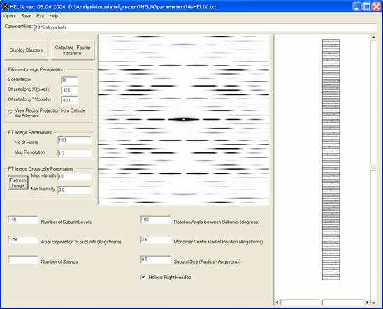
Figure 10: Simulation of diffraction from an 18/5 Alpha-helix
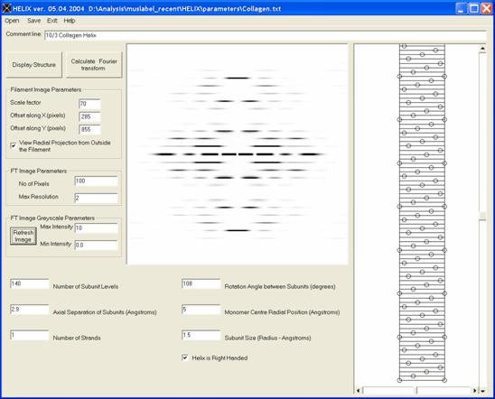
Figure 11: Simulation of diffraction from a collagen 10/3 helix
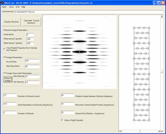
Figure 12: Simulation of diffraction from a 3-stranded 9/1 myosin filament
TABLE 1: Parameter values for some well-known helical structures for use in simulations generated by the HELIX program.
|
STRUCTURE | B-DNA | A-DNA | Collagen 10/3 | 3 Stranded Myosin Filament | 13/6 Actin Filament | 18/5 Alpha-HELIX |
| (A) Structure Parameters |
|
|
|
|
|
|
| Axial separation (h) of subunits (Å) |
3.4 | 2.54 | 2.9 | 143 | 27.5 | 1.49 |
| Rotation (f ) between subunits (degrees) | 36 | 32.7 |
108 | 40 | 166.154 | 100 |
| Monomer centre radial (r) position (Å) | 7 | 9 | 5 | 150 | 25 | 2.5 |
| Monomer subunit size (Å) | 1.2 | 1.5 | 30 | 10 | 0.5 | |
| Hand of helix | RH | RH | RH | RH | LH | RH |
| No of subunit levels | 50 | 140 | 140 | 100 | 100 | 140 |
| No of strands | 2 | 2 | 1 | 3 | 1 | 1 |
| If No of strands = 2 |
|
| ||||
| Azimuthal shift of strand 2 (degrees) | 143 | 170 |
N/A | N/A |
N/A | N/A |
| Axial shift of strand 2 (Å) | 0 |
2 |
N/A |
N/A |
N/A |
N/A |
|
(B) Display Parameters
|
|
|
|
| ||
|
Scale factor |
60 |
50 |
2 |
100 |
100 | |
| Offset along X (Pixels) | 240 | 230 | 255 | 250 | 275 | 255 |
| Offset along Y (Pixels) | 645 | 685 | 690 | 680 | 695 | 690 |
|
(C) Transform Parameters
|
|
|
|
|
|
|
|
No of Pixels |
100 |
100 |
100 |
100 |
100 |
100 |
| Max resolution (Å) | 2.5 | 2 | 2 | 40 | 20 | 1.3 |
| Max Intensity | 25 | 25 | 10 | 15 | 25 | 25 |
| Min Intensity | 0 | 0 | 0 | 0 | 0 | 0 |
Exercises
The features of the diffraction patterns are very sensitive to the parameters describing the model structures. Using HELIX, it is possible to explore the effects on the diffraction pattern when the structure parameters are changed. For example, starting from the parameter file describing B-DNA, it is interesting to find out:
- What happens when the radius of the spheres representing the subunits is increased or decreased?
- What are the effects on the layer lines, when the number of subunits levels is changed?
- How does the cross-like pattern outlined by the most intense reflections in the diffraction pattern change when the radial position of the centres of the monomers is varied?
- How does the pattern change when the axial separation of the monomers is changed?
- What is the effect of changing the pitch of the helix (e.g. by changing the rotation angle between subunits)?
Bibliography
An explanation for these and other effects can be found in the articles
“Fibre and Muscle Diffraction” by J.M Squire (2000) in “Structure and Dynamics of Biomolecules”, E. Fanchon, E. Geissler, L-L Hodeau, J-R Regnard & P. Timmins Eds.,Oxford University Press,
Time-resolved studies of muscle using synchrotron radiation. Harford, J.J.& Squire, J.M. (1997) Rep. Prog. Phys. 60, 1723-1787.
Use of X-ray diffraction in the study of protein and nucleic acid structure Holmes, K.C. & Blow, D.M. (1965) Interscience Publishing Company.
and in Chapter 2 of:
“The Structural Basis of Muscular Contraction ”, by Squire, J.M. (1981) Plenum press, New York and London
Contacts
Carlo Knupp ([email protected])
Biophysics Group, Dept of Optometry and Vision Sciences, Redwood Building , Cardiff University , Cardiff CF10 3NB.
John M. Squire ([email protected])
Biological Structure & Function Section, Biomedical Sciences Division, Imperial College London, London SW7 2AZ ,UK.

Diamond Light Source is the UK's national synchrotron science facility, located at the Harwell Science and Innovation Campus in Oxfordshire.
Diamond Light Source Ltd
Diamond House
Harwell Science & Innovation Campus
Didcot
Oxfordshire
OX11 0DE
Copyright © Diamond Light Source. Diamond Light Source® and the Diamond logo are registered trademarks of Diamond Light Source Ltd
Registered in England and Wales at Diamond House, Harwell Science and Innovation Campus, Didcot, Oxfordshire, OX11 0DE, United Kingdom. Company number: 4375679. VAT number: 287 461 957. Economic Operators Registration and Identification (EORI) number: GB287461957003.