
Email: [email protected]
Tel: +44 (0)1235 56 7675
Information such as the pattern centre, detector orientation, fibre tilt can be estimated and refined and putative unit cells can be plotted over the pattern. In addition, more general functions are available such as the capability to plot and fit integrated slices or scans through the pattern.
The middle part contains the large scrolled image area, the magnified area, two text fields for specifying the current display thresholds, two push buttons for inverting the current palette and refreshing the display and a set of toggle buttons used to specify subsequent behaviour and use of the pointer and mouse buttons.
The bottom part contains a scrolled text window for displaying output from the processing program, FIX and commands sent to FIX by the XFIX interface.
Lines and scans can be plotted and fitted using many of the interfaces developed for the XFIT program which utilizes PGPLOT graphics. Plotting is activated using the "Plot Lines/Scans" button in the "Process" menu. In the following description, where the word "line" is used, "scan" could be substituted.
When a line is plotted the distance between the start and end points of the line is divided into a sequence of channels, the length of a channel corresponding to the size of a data pixel. The values placed into the channels are found by interpolation of the data values. The first and last channels for plotting can be entered in the Channel Dialog box which appears soon after plotting has been activated. Clicking on the "Cancel" button in the Channel Dialog box will cause XFIX to move on to the next line selected for plotting.
When the data for the line are plotted, the thresholds for the plot will be the minimum and maximum channel values present in the selected channels. If necessary, these can be altered by entering the appropriate values into the Threshold dialog box. Clicking on the "Cancel" button in the Threshold Dialog box will cause XFIX to move on to the next line selected for plotting.
If the data is to be fitted ("Fit Lines/Scans" has been selected in the "Options" menu), the user can choose to delimit the region to be used in the fit using the Limit Dialog box. The limits can then be selected by clicking on the plot with any mouse button. Once the limits of the region have been selected, the plot will be redrawn using only the required region.
Six peak types are available:
| Peak type | Key | Parameters |
|---|---|---|
| Gaussian | g | 3 |
| Lorentzian | c | 3 |
| Pearson VII | p | 4 |
| Voigt | v | 4 |
| Debye Gaussian chain scattering | d | 3 |
| Double exponential | x | 4 |
The selection is made by pressing the appropriate key while the focus is in the plot window. All subsequent peaks will be of the same type until a different peak type is selected. The default peak type is Gaussian.
The formulae used for the different peak types give different meanings to the descriptions width and shape. In what follows, the position of the peak is assumed to be at the origin of the x-axis, h is the height of the peak, w is the width and s is the shape. Peak widths are the full width at half maximum (FWHM) unless otherwise stated.
An approximation is used:
i=14
where the constants have the following values,
| i = | 1 | 2 | 3 | 4 |
|---|---|---|---|---|
| A | -1.2150 | -1.3509 | -1.2150 | -1.3509 |
| B | 1.2359 | 0.3786 | -1.2359 | -0.3786 |
| C | -0.3085 | 0.5906 | -0.3085 | 0.5906 |
| D | 0.0210 | -1.1858 | -0.0210 | 1.1858 |
A peak of the current type is initialized for fitting to the data when the left mouse button is pressed. The position of the peak is determined by the X coordinate of the cursor when the button is pressed. The width of the peak is determined simultaneously by the Y coordinate of the cursor. The height of the peak is given by the Y value of the data point nearest to the peak position.
A polynomial of degree 4 or less, expressed as
0 + a1x + a2x2 + a3x3 + a4x4
can be fitted as background to the data. The degree of the polynomial can be selected by using the keys <1>,...,<4> while the focus is in the plot window. The default polynomial degree is 3.
An exponential component can be added into the background by pressing <e> while the focus is in the plot window. This will add two parameters to the fit to define the exponential curve,
1ee2x .
Once all the required peak and background parameters have been initialized, selection can be terminated by clicking on the right mouse button while the focus is in the plot window.
Some control over the fitting procedure can be excercised through the Setup Dialog box. This interface provides a list of all the parameters in the fit with their current values displayed in text fields so that they can be easily modified. There is also an option menu associated with each parameter. The following selections can be made from this menu:
The three buttons at the bottom of the Setup dialog box have the following effects:
The algorithm is deemed to have converged when the following two conditions are fulfilled:
Clicking on "Yes" in the "Try Again" Confirm Dialog box will give you another attempt at fitting the current frame starting from the point where you select the peak types, positions, etc. The Setup Dialog box will disappear and the Information Dialog box will appear, reiterating the procedure for setting up the initial model. Clicking on "No" will cause XFIX to proceed onto the next line.
There are three methods for estimating the background component of the diffraction pattern using XFIX:
(a) Paul Langan's "roving window" method.
(b) Calculation of a circularly-symmetric background.
(c) Calculation of a "smoothed" background through iterative low-pass filtering based on the method of M.I. Ivanova and L. Makowski (Acta Cryst. (1998) A54, 626-631).
These can be selected from the process menu by clicking on "background". All three methods require the user to input the pattern centre and the extent of the pattern (minimum and maximum radii in pixel units) in relation to the centre. Pixel values outside these limits will be ignored in the background estimation. If the diffraction pattern is not circular and centred around a single point, then it is possible to discard values less than a user-input minimum so that, for example, all values less than or equal to 0.0 are ignored in the background calculation. By using the BSL program from the NCD sofware suite , it is possible to mask the areas of the image that are not of interest (for example setting unwanted pixel values to a large negative value) and discarding these values in the background calculation.
The details of the different background estimation techniques are discussed below. In each case, once processing is completed, the user is prompted to view the calulated background. This will open a new XFIX interface with a 2-frame BSL file loaded (of filename specified by the user). This may take a few seconds. The first frame in this file is the estimated background and the next frame is the diffraction data with the calculated background subtracted. This provides a visual indication of the "goodness of fit" of the calculated background. The calculated background in frame 1 of the file can then processed further using any of the three background estimation techniques. In this way, different background subtraction methods can be used successively if desired. Finally, the data-background frame can be used with a data fitting program such as LSQINT to measure the reflection intensities.
It should be noted that these methods of background estimation can be very time-consuming when used with a large image (eg. 2000x200 pixels). It may often be worthwhile to scale down the dimensions of the diffraction pattern using XCONV (eg. to 200x200 pixels) to find the optimum parameters to be used in the process before operating on the full-size image.
The roving window background subtraction method of Paul Langan estimates the background by moving a window (of size input by the user) across the collected data. The pixel values within this window are sorted and those in the user-selected range are taken as background (except pixel values lying outside the pattern extents or specified by the user as values to discard). The average pixel value within this range is then assigned to be the estimated background at the centre of the window. Fiinally, a smoothing spline under tension is fitted to fill in the gaps between window centres. The following parameters must be input by the user:
The pattern centre in X and Y (values in pixel units).
The pattern extents taken radially from the centre (values in pixel units).
Pixel values to discard.
The window width and height (values in pixel units). The window will be of size 2*width+1 in X and 2*height+1 in Y.
The separation of the window centres in X and Y (values in pixel units).
The start and end positions in the sorted pixel list for selecting pixels corresponding to the background (expressed as a percentage of the total number of pixels in the window).
The smoothing and tension factors for the spline fitting.
The output BSL file name.
A circularly-symmetric background can be formed by the radial binning of pixel values followed by averaging those pixel values lying within a specified range. This average value is assigned to the particular radius and a smoothing spline under tension is fitted to yield the estimated background. The following parameters must be input by the user:
The pattern centre in X and Y (values in pixel units).
The pattern extents taken radially from the centre (values in pixel units).
Pixel values to discard.
The increment for radial binning (in pixel units).
The start and end positions in the sorted pixel list for selecting pixels corresponding to the background (expressed as a percentage of the total number of pixels corresponding to the radial bin).
The smoothing and tension factors for the spline fitting.
The output BSL file name.
This method of background subtraction is based on that of M.I. Ivanova and L. Makowski (Acta Cryst. (1998) A54, 626-631). It takes advantage of the fact that the background of a fibre diffraction pattern is typically composed of lower spatial frequencies than the diffraction maxima. Hence an iterative low-pass filter can be applied to separate the two components on the basis of their frequencies. The estimated background depends on the frequency limit of the filter in both X and Y.
The application of the low pass filter is achieved by the convolution of the observed diffraction pattern with a box car or gaussian function (the smoothing function) having an average value of unity taken over the number of pixels it occupies and a value of zero elsewhere. This function is convoluted with the real data at each pixel within the pattern limits (excluding pixels that are specified by the user as to be discarded). The result of applying this filter is an overestimated background, containing some intensity from the diffracted maxima. This overestimated background is then subtracted from the real data to leave the diffraction maxima whose intensities are now underestimated. Positive pixel values in the image resulting from this subtraction are then subtracted from the original data to yield the next estimate of the background. This is then convoluted with the smoothing function and the procedure is repeated, with images of the original data minus estimated background providing a visual indication of the "goodness of fit" of the estimated background. The procedure is illustrated graphically in one-dimension in Figure 1 below.
There are problems that exist with this method of background estimation at the edge of the pattern where information cannot be obtained for the convolution. This can lead to edge effects (typically an underestimation of the background) which become more pronounced with each cycle of filtering. In this case, it is possible to import a background calculated by another method to be used as the final background estimate at the edges of the pattern. This is then left as constant throughout each cycle of filtering. The backgrounds calculated by the different methods are then merged by fitting a smoothing spline under tension.
The following parameters must be input by the user:
The pattern centre in X and Y (values in pixel units).
The pattern extents taken radially from the centre (values in pixel units).
Pixel values to discard.
Whether to use a box car or gaussian as the smoothing function.
The box car size or gaussian full-width-half-maximum (FWHM) (values in pixel units).
The number of filtering cycles.
Whether to apply the smoothing function / filter at the edge of the pattern.
The background to be imported if the filter is not to be applied at the edge of the pattern.
Whether to merge the backgrounds calculated by different methods.
The smoothing and tension factors for spline fitting and the weight to be applied to the imported background in relation to the "smoothed" background.
The output BSL file name.
Once the background estimation process has been completed, the user will be prompted to view the estimated background and original pattern minus estimated background as described above. This will open a new XFIX interface ( this may take a few seconds). Once the estimated background has been inspected, the user may then choose to perform more iterations of filtering. Hence it is possible to view the estimated background after each iteration if desired.
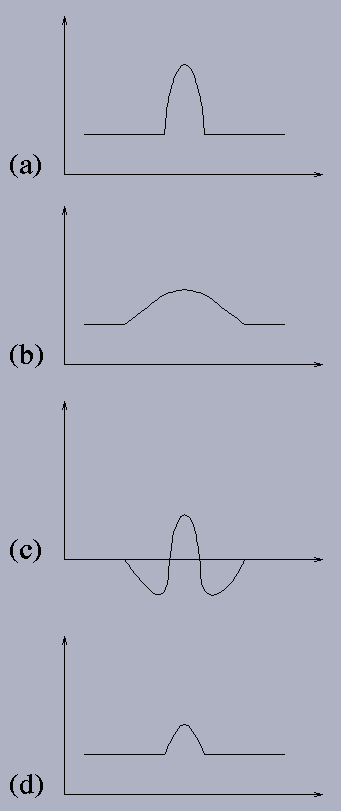
Figure 1: An illustration of the results of applying an iterative low-pass filter to the observed diffraction data.
(a) shows the current estimate of the background. On the first iteration, this is the recorded data.
(b) shows the result of "smoothing" the current background in (a) by applying a low-pass filter (ie. by convoluting the data in (a) with the smoothing function).
(c) shows the result of subtracting (b) from the original data.
(d) shows the result of subtracting positive values in (c) from the original data. (d) is now set to the current background and the procedure is repeated.
(i) Enter the wavelength & sample-detector distance under Edit/Parameters. Note that the sample-detector distance should be in pixel units. If you wish to use a calibration ring to determine this distance, see below.
(ii) Get rough values for the centre by measuring points on a salt ring, for example. If there isn't a salt ring, take four symmetry related reflections/diffraction features. Then go to Estimate/Centre. You will be asked if you want to calculate the sample-detector distance - say no unless you are dealing with a calibration ring (if so, you need to have placed the d-spacing for this ring under Edit/Parameters).
(iii) Get rough value for the rotation of sample relative to detector. Collect points in pairs, each pair containing symmetry related points on either side of MERIDIAN. Go to Estimate/Rotation.
(iv) Get rough value for the tilt of the sample relative to the x-ray beam. Collect points in pairs, each pair containing symmetry related points on either side of EQUATOR. Go to Estimate/Tilt. Remember this is a sensitive calculation (tangent changing very fast) where small measurement errors have a substantial effect. Your initial value may not be that good.
(v) Now refine the parameters (see Process/Refine). The refinement works by minimising the variance of the current selected region for all four quadrants (as defined in reciprocal space), and then using a downhill simplex algorithm for refinement. It usually works well but you have to be careful.
In zoom mode select a small(ish) box that looks promising. I have always found that the best approach is to refine centre & rotation first using a zoom box with clear features on all four quadrant, in a region that is not specifically affected by tilt. Then go to Process/Refine and activate "centre" and "Detector rotation", followed by "OK". If the selected region is not too large, the refinement will be quite quick.
Following this choose a region of the pattern for which tilt is clearly important (usually close to meridian, fairly high in Z) and for which symmetry related data are available in all four quadrants. Go to Process/Refine and activate "Specimen Tilt" only, followed by "OK".
Once you have these, you can try to refine things together. The last step is to try detector tilt & twist.
(vi) Once you have the parameters well determined to can try the background subtraction - eg (Process/Background) and then proceed to the RZ mapping step in FTOREC.

Diamond Light Source is the UK's national synchrotron science facility, located at the Harwell Science and Innovation Campus in Oxfordshire.
Copyright © 2022 Diamond Light Source
Diamond Light Source Ltd
Diamond House
Harwell Science & Innovation Campus
Didcot
Oxfordshire
OX11 0DE
Diamond Light Source® and the Diamond logo are registered trademarks of Diamond Light Source Ltd
Registered in England and Wales at Diamond House, Harwell Science and Innovation Campus, Didcot, Oxfordshire, OX11 0DE, United Kingdom. Company number: 4375679. VAT number: 287 461 957. Economic Operators Registration and Identification (EORI) number: GB287461957003.

 Soft Condensed Matter - Small Angle Scattering